Plotting of scale-dependent features.

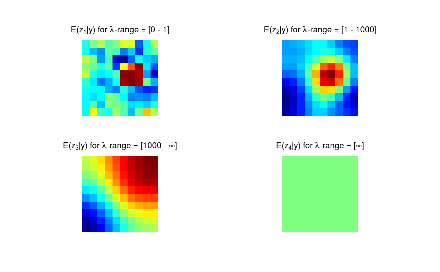
Scale-dependent features are plotted using differences of smooths at neighboring scales. The features are summarized by their posterior mean.

# S3 method for smMeanGrid
plot(x, color.pallet = fields::tim.colors(),
  turnOut = TRUE, title, aspRatio = 1, ...)

Arguments

x	List containing the posterior mean of all differences of smooths.
color.pallet	The color pallet to be used for plotting scale-dependent features.
turnOut	Logical. Should the output images be turned 90 degrees counter-clockwise?
title	Vector containing one string per plot. The required number of titles is equal to length(mrbOut$smMean). If no title is passed, defaults are used.
aspRatio	Adjust the aspect ratio of the plots. The default aspRatio = 1 produces square plots.
...	Further graphical parameters can be passed.

Value

Plots of the differences of smooths are created.

Details

x corresponds to the smmean-part of the output of mrbsizeRgrid.

Examples

# Artificial sample data
set.seed(987)
sampleData <- matrix(stats::rnorm(100), nrow = 10)
sampleData[4:6, 6:8] <- sampleData[4:6, 6:8] + 5

# Generate samples from multivariate t-distribution
tSamp <- rmvtDCT(object = sampleData, lambda = 0.2, sigma = 6, nu0 = 15,
                   ns = 1000)

# mrbsizeRgrid analysis
mrbOut <- mrbsizeRgrid(posteriorFile = tSamp$sample, mm = 10, nn = 10,
                       lambdaSmoother = c(1, 1000), prob = 0.95)

# Posterior mean of the differences of smooths
plot(x = mrbOut$smMean, turnOut = TRUE)