Plotting of scale-dependent features on a sphere.

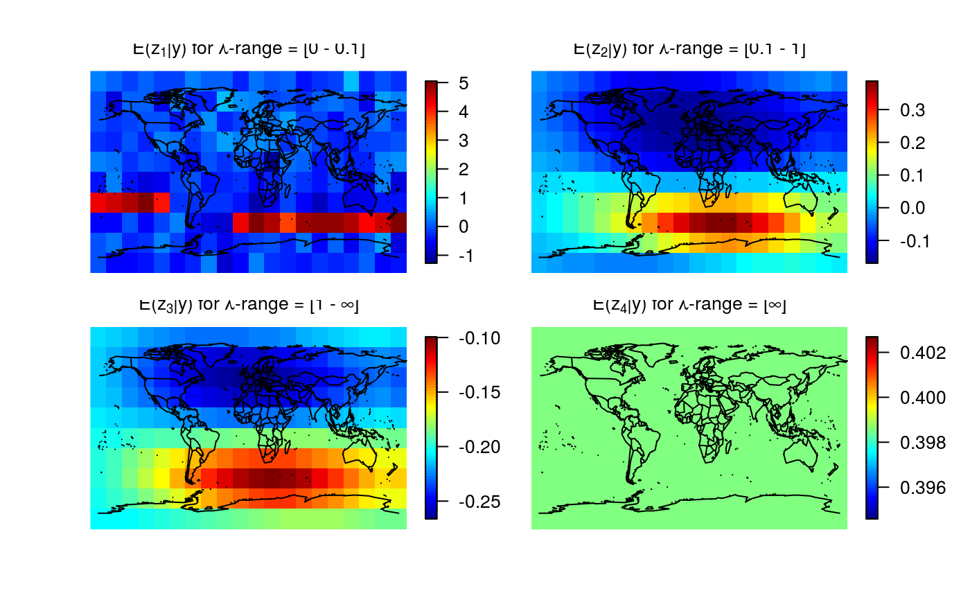
Scale-dependent features are plotted using differences of smooths at neighboring scales. The features are summarized by their posterior mean. Continental lines are added to the plots.

# S3 method for smMeanSphere
plot(x, lon, lat,
  color.pallet = fields::tim.colors(), turnOut = TRUE, title, ...)

Arguments

x	List containing the posterior mean of all differences of smooths.
lon	Vector containing the longitudes of the data points.
lat	Vector containing the latitudes of the data points.
color.pallet	The color pallet to be used for plotting scale-dependent features.
turnOut	Logical. Should the output images be turned 90 degrees counter-clockwise?
title	Vector containing one string per plot. The required number of titles is equal to length(mrbOut$smMean). If no title is passed, defaults are used.
...	Further graphical parameters can be passed.

Value

Plots of the differences of smooths are created.

Details

x corresponds to the smmean-part of the output of mrbsizeRsphere.

Examples

# Artificial spherical sample data
set.seed(987)
sampleData <- matrix(stats::rnorm(2000), nrow = 200)
sampleData[50:65, ] <- sampleData[50:65, ] + 5
lon <- seq(-180, 180, length.out = 20)
lat <- seq(-90, 90, length.out = 10)

# mrbsizeRsphere analysis
mrbOut <- mrbsizeRsphere(posteriorFile = sampleData, mm = 20, nn = 10,
                         lambdaSmoother = c(0.1, 1), prob = 0.95)

# Posterior mean of the differences of smooths
plot(x = mrbOut$smMean, lon = lon, lat = lat,
     color = fields::tim.colors(), turnOut = FALSE)